In 1921 Albert Wallace Hull invented the
magnetron as a powerful microwave tube.
Magnetrons function as self-excited microwave
oscillators. Crossed electron and magnetic fields are used in the magnetron
to produce the high-power output required in radar equipment. These
multicavity devices may be used in radar transmitters as either pulsed or cw
oscillators at frequencies ranging from approximately 600 to
30,000 megahertz. The relatively simple construction has the disadvantage,
that the Magnetron usually can work only on a constructively fixed
frequency.
Physical construction of a magnetron
The magnetron is classed as a diode because
it has no grid. The anode of a magnetron is fabricated into a cylindrical
solid copper block. The cathode and filament are at the center of the tube
and are supported by the filament leads. The filament leads are large and
rigid enough to keep the cathode and filament structure fixed in position.
The cathode is indirectly heated and is constructed of a high-emission
material. The 8 up to 20 cylindrical holes around its circumference are
resonant cavities. The cavities control the output frequency. A narrow slot
runs from each cavity into the central portion of the tube dividing the
inner structure into as many segments as there are cavities.
| |
resonant cavities |
anode |
|
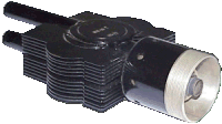
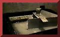
Figure 2: Magnetron МИ 29Г of the Bar Lock |
| filament leads |
 |
cathode
pickup loop |
| Figure 1: Cutaway view of a magnetron |
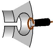
The open space between the plate and the
cathode is called the interaction space. In this space the electric and
magnetic fields interact to exert force upon the electrons. The magnetic
field is usually provided by a strong, permanent magnet mounted around the
magnetron so that the magnetic field is parallel with the axis of the
cathode.
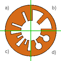
Figure 3: forms of the plate of magnetrons |
|
The form of the cavities varies, shown in the
Figure 3. The output lead is usually a probe or loop extending into
one of the tuned cavities and coupled into a waveguide or coaxial
line. |
a) slot- type
b) vane- type
c) rising sun- type
d) hole-and-slot- type |
Basic Magnetron Operation
As when all velocity-modulated tubes the
electronic events at the production microwave frequencies at a Magnetron can
be subdivided into four phases too:
- phase: Production and acceleration of an electron beam
- phase: Velocity-modulation of the electron beam
- phase: Forming of a �Space-Charge Wheel�
- phase: Giving up energy to the ac field
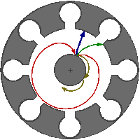
Figure 4: the electron path under the influence of the
varying magnetic field. |
|
1. Phase Production and acceleration of an
electron beam
When no magnetic field exists, heating the cathode
results in a uniform and direct movement of the field from the
cathode to the plate (the blue path in figure 4). The permanent
magnetic field bends the electron path. If the electron flow reaches
the plate, so a large amount of plate current is flowing. If the
strength of the magnetic field is increased, the path of the
electron will have a sharper bend. Likewise, if the velocity of the
electron increases, the field around it increases and the path will
bend more sharply. However, when the critical field value is
reached, as shown in the figure as a red path, the electrons are
deflected away from the plate and the plate current then drops
quickly to a very small value. When the field strength is made still
greater, the plate current drops to zero.
When the magnetron is adjusted to the cutoff, or critical value
of the plate current, and the electrons just fail to reach the plate
in their circular motion, it can produce oscillations at microwave
frequencies. |
2. Phase: velocity-modulation of the electron beam
The electric field in the magnetron
oscillator is a product of ac and dc fields. The dc field extends radially
from adjacent anode segments to the cathode. The ac fields, extending
between adjacent segments, are shown at an instant of maximum magnitude of
one alternation of the rf oscillations occurring in the cavities.
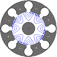
Figure 5: The high-frequency electrical field |
|
In the figure 5 is shown only the assumed
high-frequency electrical ac field. This ac field work in addition
to the to the permanently available dc field. The ac field of each
individual cavity increases or decreases the dc field like shown in
the figure.
Well, the electrons which fly toward the anode
segments loaded at the moment more positively are accelerated in
addition. These get a higher tangential speed. On the other hand the
electrons which fly toward the segments loaded at the moment more
negatively are slow down. These get consequently a smaller
tangential speed. |
3. Phase: Forming of a �Space-Charge Wheel�
On reason the different speeds of the
electron groups a velocity modulation appears therefore.
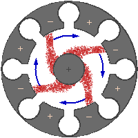
Figure 6: Rotating space-charge
wheel in an eight-cavity magnetron |
|
The cumulative action of many electrons returning
to the cathode while others are moving toward the anode forms a
pattern resembling the moving spokes of a wheel known as a
�Space-Charge Wheel�, as indicated in figure 6. The space-charge
wheel rotates about the cathode at an angular velocity of 2 poles
(anode segments) per cycle of the ac field. This phase relationship
enables the concentration of electrons to continuously deliver
energy to sustain the rf oscillations.
One of the spokes just is
near an anode segment which is loaded a little more negatively. The
electrons are slowed down and pass her energy on to the ac field.
This state isn't static, because both the ac- field and the wire
wheel permanently circulate. The tangential speed of the electron
spokes and the cycle speed of the wave must be brought in agreement
so.
|
4. Phase: Giving up energy to the ac field
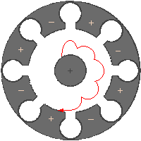
Figure 7: Path of an electron |
|
Recall that an electron moving against an E field
is accelerated by the field and takes energy from the field. Also,
an electron gives up energy to a field and slows down if it is
moving in the same direction as the field (positive to negative).
The electron gives up energy to each cavity as it passes and
eventually reaches the anode when its energy is expended. Thus, the
electron has helped sustain oscillations because it has taken energy
from the dc field and given it to the ac field. This electron
describes the path shown in figure 7 over a longer time period
looked. By the multiple breaking of the electron the energy of the
electron is used optimally. The effectiveness reaches values up to
80%. |
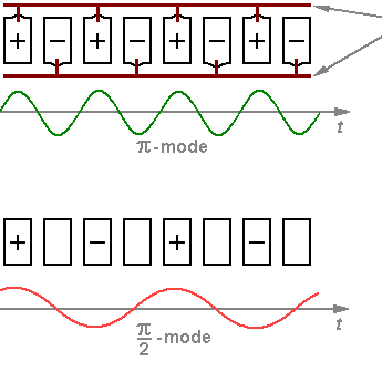
Modes of Oscillation
The operation frequency depends on the
measurements of the cavities and the interaction space between anode and
cathode. But the single cavities are coupled over the interaction space with
each other. Therefore several resonant frequencies exist for the complete
system. Two of the four possible waveforms of a magnetron with 8 cavities
are in the figure 8 represented. Several other modes of oscillation are
possible (3/4π, 1/2π, 1/4π), but a magnetron operating
in the π mode has greater power and output and is the most commonly
used.
 |
|
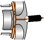
Strapping
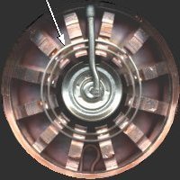
Figure 9: cutaway view of a magnetron, showing the
strapping rings and the slots.
Figure 8: Waveforms of the magnetron
(Anode segments are represented �unwound�) |
So that a stable operational condition adapts
in the optimal pi mode, two constructive measures are possible:
- Strapping rings:
The frequency of the π mode is separated from the frequency of
the other modes by strapping to ensure that the alternate segments have
identical polarities. For the pi mode, all parts of each strapping ring
are at the same potential; but the two rings have alternately opposing
potentials. For other modes, however, a phase difference exists between
the successive segments connected to a given strapping ring which causes
current to flow in the straps.
- Use of cavities of different
resonance frequency
E.g. such a variant is the anode form �Rising Sun�.
Magnetron
coupling methods
Energy (rf) can be removed from a magnetron
by means of a coupling loop. At frequencies lower than 10,000 megahertz, the
coupling loop is made by bending the inner conductor of a coaxial line into
a loop. The loop is then soldered to the end of the outer conductor so that
it projects into the cavity, as shown in figure 1, view (A). Locating the
loop at the end of the cavity, as shown in view (B), causes the magnetron to
obtain sufficient pickup at higher frequencies.
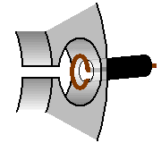
Figure 10: Magnetron coupling, view (A) |
view (B) |
The segment-fed loop method is shown in view
(C) of figure 2. The loop intercepts the magnetic lines passing between
cavities. The strap-fed loop method (view (D), intercepts the energy between
the strap and the segment. On the output side, the coaxial line feeds
another coaxial line directly or feeds a waveguide through a choke joint.
The vacuum seal at the inner conductor helps to support the line. Aperture,
or slot, coupling is illustrated in view (E). Energy is coupled directly to
a waveguide through an iris.
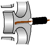
Figure 11: Magnetron coupling, view (C) |
|
view (D) |
|
view (E) |
Magnetron tuning
A tunable magnetron permits the system to be
operated at a precise frequency anywhere within a band of frequencies, as
determined by magnetron characteristics. The resonant frequency of a
magnetron may be changed by varying the inductance or capacitance of the
resonant cavities.
Tuner frame
anode block |
|
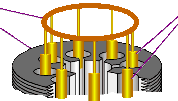
Figure 12: Inductive magnetron tuning |
|
inductive
tuning
elements |
An example of a tunable magnetron is the
M5114B used by the ATC- Radar ASR-910. To reduce mutual
interferences, the ASR-910 can work on different assigned
frequencies. The frequency of the transmitter must be tunable therefore.
This magnetron is provided with a mechanism to adjust the Tx- frequency of
the ASR-910 exactly.
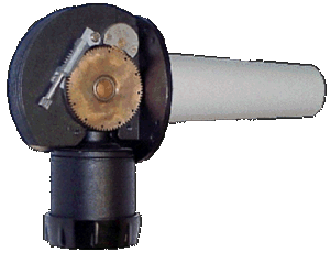
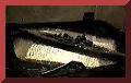
Figure 13: Magnetron M5114B of the ATC-radar ASR-910
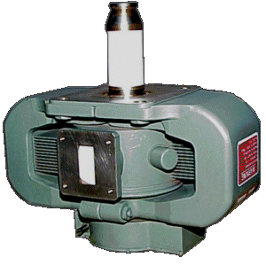
Figure 13: Magnetron VMX1090 of the ATC-radar PAR-80 This magnetron is even equipped with the permanent magnets necessary for the
work.